Pixels to Profits: The Evolution of Global Gaming

Code

# Loading required libraries
library(tidyverse)
library(plotly)
library(gganimate)
library(hrbrthemes)
library(gifski)

# Loading and Cleaning Data
vgsales <- read_csv("/Users/marcusjabari/Downloads/vgsales.csv") %>%
  filter(!is.na(Year), Year <= 2016) %>%
  mutate(Year = as.numeric(Year))


# Reshaping data for regional analysis
vgsales_long <- vgsales %>%
  pivot_longer(cols = c(NA_Sales, EU_Sales, JP_Sales),
               names_to = "Region",
               values_to = "Sales") %>%
  mutate(Region = str_replace(Region, "_Sales", ""))

# Preview the transformed data
head(vgsales_long) %>% knitr::kable()

Rank	Name	Platform	Year	Genre	Publisher	Other_Sales	Global_Sales	Region	Sales
1	Wii Sports	Wii	2006	Sports	Nintendo	8.46	82.74	NA	41.49
1	Wii Sports	Wii	2006	Sports	Nintendo	8.46	82.74	EU	29.02
1	Wii Sports	Wii	2006	Sports	Nintendo	8.46	82.74	JP	3.77
2	Super Mario Bros.	NES	1985	Platform	Nintendo	0.77	40.24	NA	29.08
2	Super Mario Bros.	NES	1985	Platform	Nintendo	0.77	40.24	EU	3.58
2	Super Mario Bros.	NES	1985	Platform	Nintendo	0.77	40.24	JP	6.81

The History of Growth

The gaming industry saw a massive explosion in the mid-2000s, driven by the “Casual Gaming” revolution led by the Nintendo Wii.

##Animated Trend (1980 - 2016) The following animation shows the “Golden Age of Growth,” highlighting the dramatic spike in global units sold.

Code

# Preparing data for animation
annual_trend <- vgsales %>%
  group_by(Year) %>%
  summarize(Total_Sales = sum(Global_Sales))

# Creating animated plot
p_anim <- ggplot(annual_trend, aes(x = Year, y = Total_Sales, group = 1)) + # Added group = 1
  geom_line(color = "steelblue", size = 1) +
  geom_point(color = "steelblue", size = 2) +
  theme_minimal() +
  scale_x_continuous(breaks = seq(1980, 2016, by = 5)) +
  labs(title = "Annual Global Game Sales",
       subtitle = "Year: {frame_along}",
       y = "Millions of Units",
       x = "Year") +
  transition_reveal(Year)

# To make it show up in Quarto, call the object explicitly:
animate(p_anim, renderer = gifski_renderer())

Market Leaders Who dominates the sales charts? By creating an interactive visualization, we can explore the top 10 best-selling games of all time and see the impact of console bundling.

Interactive Top 10 Best Sellers Hover over the bars to see specific sales figures and publishers.

Code

top_10 <- vgsales %>%
  slice_max(Global_Sales, n = 10)

p_interact <- ggplot(top_10, aes(x = reorder(Name, Global_Sales), 
                                 y = Global_Sales, 
                                 fill = Platform,
                                 text = paste("Game:", Name, 
                                              "<br>Sales:", Global_Sales, "M",
                                              "<br>Publisher:", Publisher))) +
  geom_col() +
  coord_flip() +
  theme_minimal() +
  labs(title = "Top 10 Global Best Sellers",
       x = "",
       y = "Global Sales (Millions)")

ggplotly(p_interact, tooltip = "text")

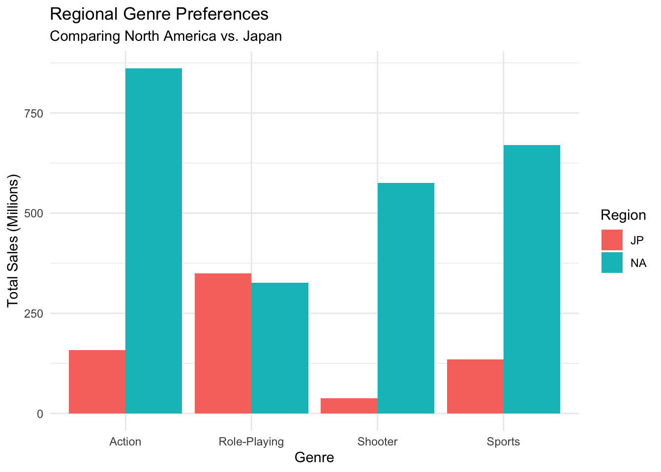
Regional Insights

One of the most interesting findings is the cultural gap between North America and Japan. While the West is driven by Action and Shooter games, Japan remains the global stronghold for Role-Playing Games.

Code

vgsales_long %>%
  filter(Region %in% c("NA", "JP"), 
         Genre %in% c("Action", "Role-Playing", "Shooter", "Sports")) %>%
  group_by(Region, Genre) %>%
  summarize(Total_Sales = sum(Sales)) %>%
  ggplot(aes(x = Genre, y = Total_Sales, fill = Region)) +
  geom_col(position = "dodge") +
  theme_minimal() +
  labs(title = "Regional Genre Preferences",
       subtitle = "Comparing North America vs. Japan",
       y = "Total Sales (Millions)")

Conclusion The data tells a clear story: the gaming industry is not a monolith. Its success is driven by hardware innovation (the Wii effect), cultural specialization (the RPG market in Japan), and blockbuster “Mega-Hits” that define entire decades.